CAPTAIN Toolbox website
Overview & availability
User interface & examples
Time variable parameter subset
Multivariable transfer function subset
Analysis of air passenger series.
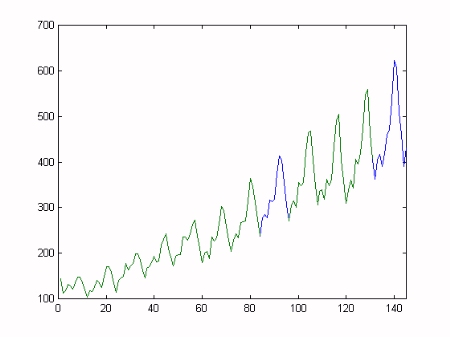
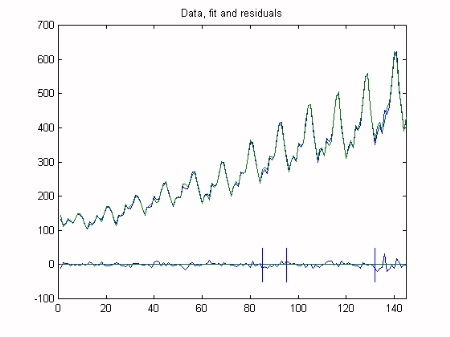
Dynamic Harmonic Regression (DHR) analysis is particularly useful for signal extraction and forecasting for periodic or quasi-periodic series. As we shall see below, it provides smoothed estimates of the series, as well as all its components (trend, fundamental frequency and harmonic components), together with the estimated changing amplitude and phase of the latter. Here, we utilise the Captain Toolbox to analyse the famous monthly air passenger time series (1949-1960). Missing values are added to the data in order to test the ability of the algorithms to automatically handle interpolation and forecasting, i.e. samples 85-95 (interpolation) and 132-145 (forecasting) are replaced by Matlab not-a-number variables. The missing data are shown as the blue trace in the plot below.
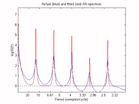
Our structural model will be composed of a trend, a 12 month (seasonal) component and the first 4 harmonics. We will assume that all of the time variable parameters vary in the form of an integrated random walk. The first stage of the analysis is to optimise the Noise Variance Ratio (NVR) hyper-parameters of the model. In the Captain Toolbox, a special frequency domain optimisation is utilsed for this task, based on fitting the DHR model pseudo-spectrum to the logarithm of the auto-regression spectrum, as illustrated below.
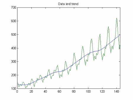
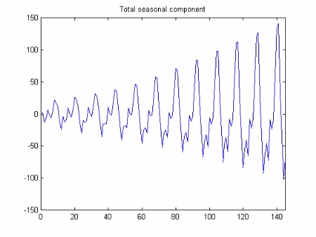
Finally, Kalman Filtering and Fixed Interval Smoothing algorithms are employed to estimate the model, based on the optimsed NVR values. This is achieved with a straightforward call to the Captain Toolbox dhr function. The trend component of the model gradually increases over time and appears to identify the business cycle. The seasonal component similarly increases over time, in order to handle the non stationarity in the series. These variables are illustrated below.
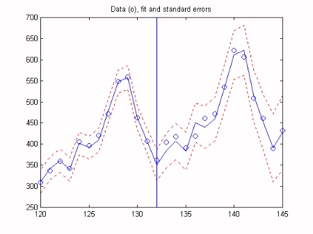
The analysis successfully interpolates over the 10 months of missing data starting at sample 85 and forecasts the series for the final year, i.e. sample 132 until the end of the series. The graph below shows the data (green), model and residuals (bottom), with the interpolation and forecasting horizons shown as the vertical bars over the residuals. The final graph is a close up view of the model for last two years of the series and shows the standard errors gradually increasing beyond the forecasting horizon. Note that the model output for the last year of the series, to the right of the vertical line, is a true 12 month forecast: these data were not employed in the analysis at any stage.
![]()
| next example |
![]()
![]()